What Makes a Painting Emotional? Using Deep Learning and Art Theory to Interpret the Emotional Character of Paintings
WenXin Dong (wxd@stanford.edu)
Leonidas Guibas (guibas@cs.stanford.edu)
Panos Achlioptas (optas@stanford.edu)
[Poster]
[GitHub]
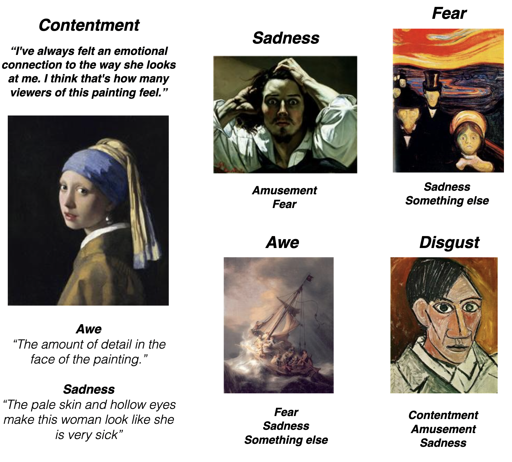
Figure 1. Examples in the ArtEmis dataset. For each painting in the ArtEmis dataset, 5 or more Amazon Turk workers provide reasoning for their dominant emotion. The majority ground truth emotion is shown above the image, and minority ground truth emotions are shown below the image.

Abstract

Paintings evoke subjective emotions. An emotion may be evoked by the semantic implication of the illustrated subject matter or the subconscious impact of nonfigurative elements to the visual system. For example, a painting of sharks may evoke fear, yet if it were drawn in bright and lively colors one might feel excited by it. Similarly, a portrait with neural expression could be interpreted as angry if hard lines and sharp angles where emphasized. It is therefore interesting from an Art Theory perspective to understand what features of a painting are more powerful at affecting the emotional responses in humans.

In this work, we find interpretations for emotional response to paintings through (1) analysing the importance of 179 handcrafted features in predicting human's dominant emotional response to paintings. Specifically, we use Art Theory and Psychology features [3, 9], low-level classical vision features [3], bounding boxes of people [15],genre [11], and art style [16]; (2) interpreting the knowledge encoded in deep learning based features.

Our findings suggest that color (hue, saturation, brightness) contrast is the most important feature in predicting the emotional response to paintings. In addition, we find that a deep CNN model was able to automatically learn the most useful low-level features, including color, texture, composition statistics. Finally, we find that by explicitly adding semantic information encoded in high-level features, we improve the naive deep model's prediction accuracy.


Key Findings

  1. Color is the most important feature category for interpreting the emotion of paintings. Top 3 most important individual features are GLCM saturation contrast (local saturation contrast), colorfulness (diversity of saturation, hue and intensity), and number of black pixels (level of intensity).

  2. Deep-learning emotion classifier successfully learns the most useful low-level features out of a list of 179 features.

  3. By explicitly adding as input the semantic information encaptured by artstyle, genre, and bounding boxes of people, we improve the naive deep learning emotion prediction accuracy.

Related work

Affective analysis is the research area that aims to identiy the emotion expressed in the input. Earlier work in affective analysis of paintings proposed handcrafted features based on psychology and Art Theory [3], the visual effect of shapes [2], principles of art [9], Itten’s color theory, texture [4], among a variety of low-level features. The main limitation of these handcrafted features is their inability at capturing global composition and semantics.

With the advance of deep learning, extracting global-level semantic features in paintings was made possible. Several deep architectures had been proposed for extracting both low-level and high-level features simultaneously. For example, Rao et al. [6] introduced a fusion model that fuses output from convolutional layers of different levels in a CNN as feature extraction; Lu et al. [7] introduced a parallel CNN architecture that takes in both the global picture and a local patch to rate pictorial aesthetics.

Few work has compared handcrafted features with deep-learning based features. You et al. [8] compared the performance between handcrafted feature sets, raw ImageNet-CNN representations, and finetuned-CNN representations, and found the deep-learning based representations to outperform handcrafted features. However, they did not analyse the correlation between handcrafted and learned features. Kim et al. [10] combined handcrafted features with the final output of a pre-trained model (object-tags) and observed improvement in classification accuracy of emotions in images.

On the line of interpreting deep representations, Elgammal el al. [11] analysed representations learned by finetuned pretrained CNN models on a style classification task using various projection methods. Côté-Allard et al. [12] analysed the relationship between handcrafted and learned features for gesture classification through employing topological data analysis, Guided Grad-CAM, and feature classification prediction. To the best of our knowledge, no work so far has focused on the interpretability of deep-learning based features for emotion classification of paintings.


Dataset

We use ArtEmis [13] as our dataset, which contains 80k WikiArt paintings with ground-truth emotion distributions. We use a subset of 30k paintings that have a dominant emotion in the ground-truth distribution. The ArtEmis dataset has 9 emotion labels: Amusement, Awe, Excitement, Contentment, Anger, Disgust, Fear, Sadness, and Something else.


Method

On a high level, we first obtain two sets of features: handcrafted features and deep-learning based features. We then compare their performance. Afterward, we calculate feature importance of the handcrafted features. Finally, we find the correlation between the handcrafted features and deep-learning based features.

Feature Engineering

To obtain deep-learning based features, we trained a ResNet-34 model from scratch, without pretrained weights. We used early stopping, 128 as batch size, 0.0005 as learning rate, and 0.3 as dropout. We extracted the output of the second to last linear layer, before the Relu nonlinearity, as our deep feature. The training task was emotion distribution prediction using a KL divergence loss. The training set was the full 80K artemis dataset.

To obtain handcrafted features, we curated 179 features from painting metadata, previous literature, and bounding boxes of people. We grouped the handcrafted features into 12 groups: hue, texture, artstyle, genre, saturation and brightness, rule of third, bounding box, faces and skin, lines, bilateral symmetry, rotational symmetry, and radial symmetry. For more detail, please see the full list of handcrafted features and their meaning.

Models

For multiclass emotion classification, we use a balanced Artemis dataset with 8 emotions. We drop the emotion class Anger due to its infrequency.

For binary emotion classification, we use a balanced binary Artemis dataset. The positive class encompasses Amusement, Awe, Excitement, Contentment, and negative class encompasses Anger,Disgust, Fear, Sadness. We drop Something Else due to its ambigouity.

We use an autoML library, Autogluon, to automatically select model family and hyperparameter.

Feature Importance

We compare two methods of calculating feature importance for the handcrafted features.

1. Classification Accuracy

Train an emotion classifier using a single feature, and approximate the feature importance using the test accuracy. This method disregards feature interactions.

2. SHAP values

SHAP values was proposed as a unified measure of feature importance for feature-based classifiers [14].In simple terms, the SHAP value of a feature represents the marginal contribution of that feature to the final prediction. It takes exponential time to calculate the true SHAP values as it requires testing all permutations of the features, and it is therefore common pratice to approximate SHAP values using samplers. The authors of SHAP introduced efficient approximation methods and we use their API in this project. SHAP assumes feature independence as correlations among features might cause features which did not contribute to the prediction to share the credits of those features that did contribute to the prediction. However, this assumption does not hold for our set of the handcrafted features, since many of them are correlated. However, independence does generally hold true for the 12 feature groups.


Finding correlation between handcrafted and deep-learning based features

We use Canonical Correlation Analysis (CCA) to find the amount of shared information between the two feature sets. Given two sets of random variables X and Y, CCA finds k pairs of canonical variables, where the first canonical variable in each pair is a linear combination of X and the second canonical varible is a linear combination of Y. CCA finds k pairs such that the two canonical variables in each pair are maximally correlated with each other, and are uncorrelated with canonical variables in the other pairs. The pairs of canonical variables are constructed iteratively. I.e. The first pair of canonical variables is calculated first, and imposes constaint on the second pair of canonical variables. One can find a maximum of min(dim(X), dim(Y)) pairs of canonical variables.

Let X be our 100D learned features, and Y be a multi-dimensional handcrafted feature group. For X and Y, we find pairs of canonical variables with significant correlation coefficient (>0.45). For each pair of canonical variables, we find the variance explained between the variables by taking the square of their correlation coefficient. We then calculate the proportion of variance shared between X and Y across all canonical variates, Rc^2. Since each pair of canonical variables aim to explain the variance that the existing pairs did not explain, each pair contribute (1- Rc^2) * (correlation_coefficient)^2 to the overall Rc^2, recursively.

Carrying out the above method for different handcrafted groups, we find the Rc^2 value for each handcrafted feature group. These Rc^2 values are used as an approximation to the proportion of variance of the feature set with smaller variance explained by the feature set with larger variance.


Results

Feature performance


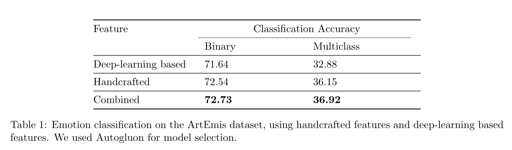
Handcrafted features outperform deep-learning based features in both binary and multiclass classification. The ourperformance margin in binary classification is 0.9% and in multiclass classification is 3.3%. Furthermore, we observe combining handcrafted features with deep-learning features gives an overall better performance in both binary and multiclass classification.

Feature importance


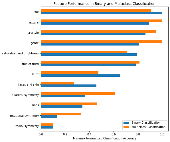
The performance of feature groups are similar in binary and multiclass classification. The top 4 feature groups with highest test accuracy are hue, texture, artstyle, and genre.


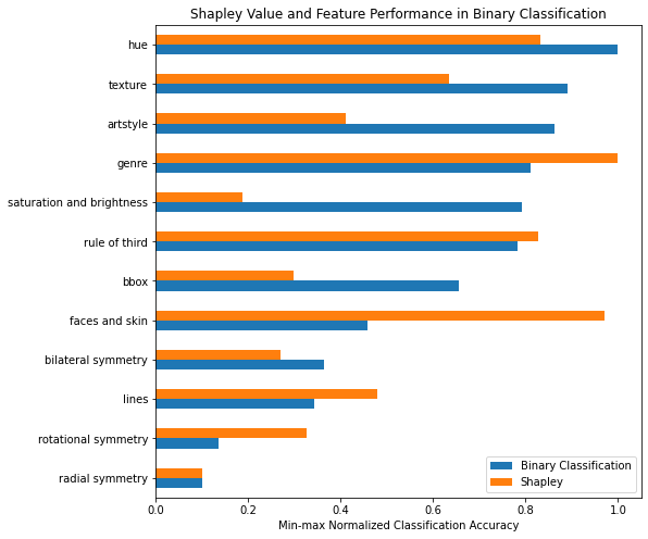
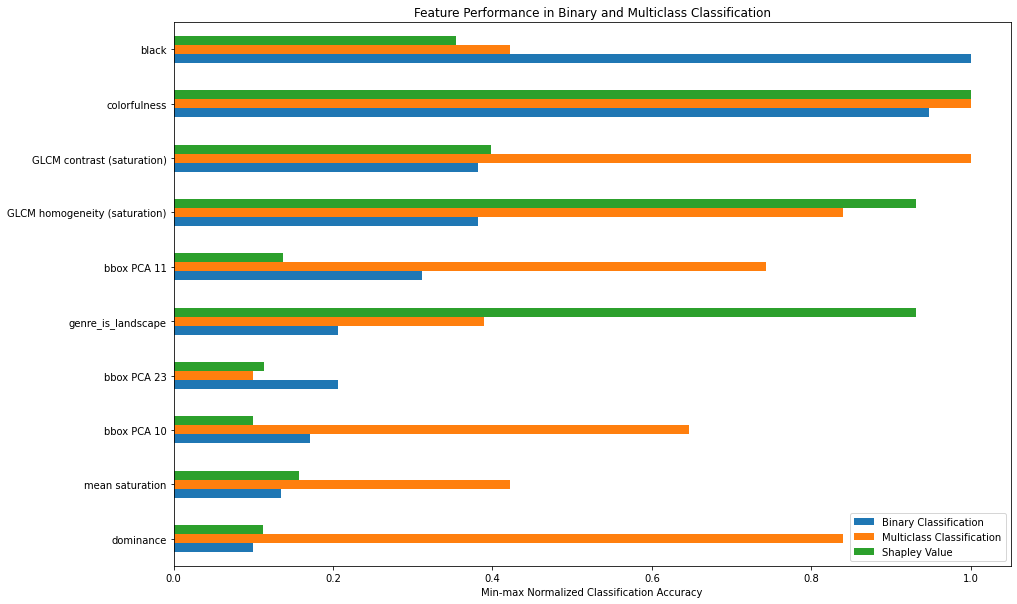
We observe feature ranking discrepancy between the Shapley value and feature performance in the binary classification setting (and a similar discrepancy in the multiclass classification setting). This might due to the fact that feature interactions are accounted for in the Shapley values but are not in feature performance. That is, some features may have larger Shapley value because they provide more information when used in conjunction with other feature groups.


Figure 2. Top 10 feature performance in Binary Classfication, and their corresponding Multiclass Classification Performance and Shapley Value.

The feature where the Binary Classification accuracy, Multiclass Classification accuracy, and Shapley value produced the most consistent result for is "colofulness".


What is colorfulness?

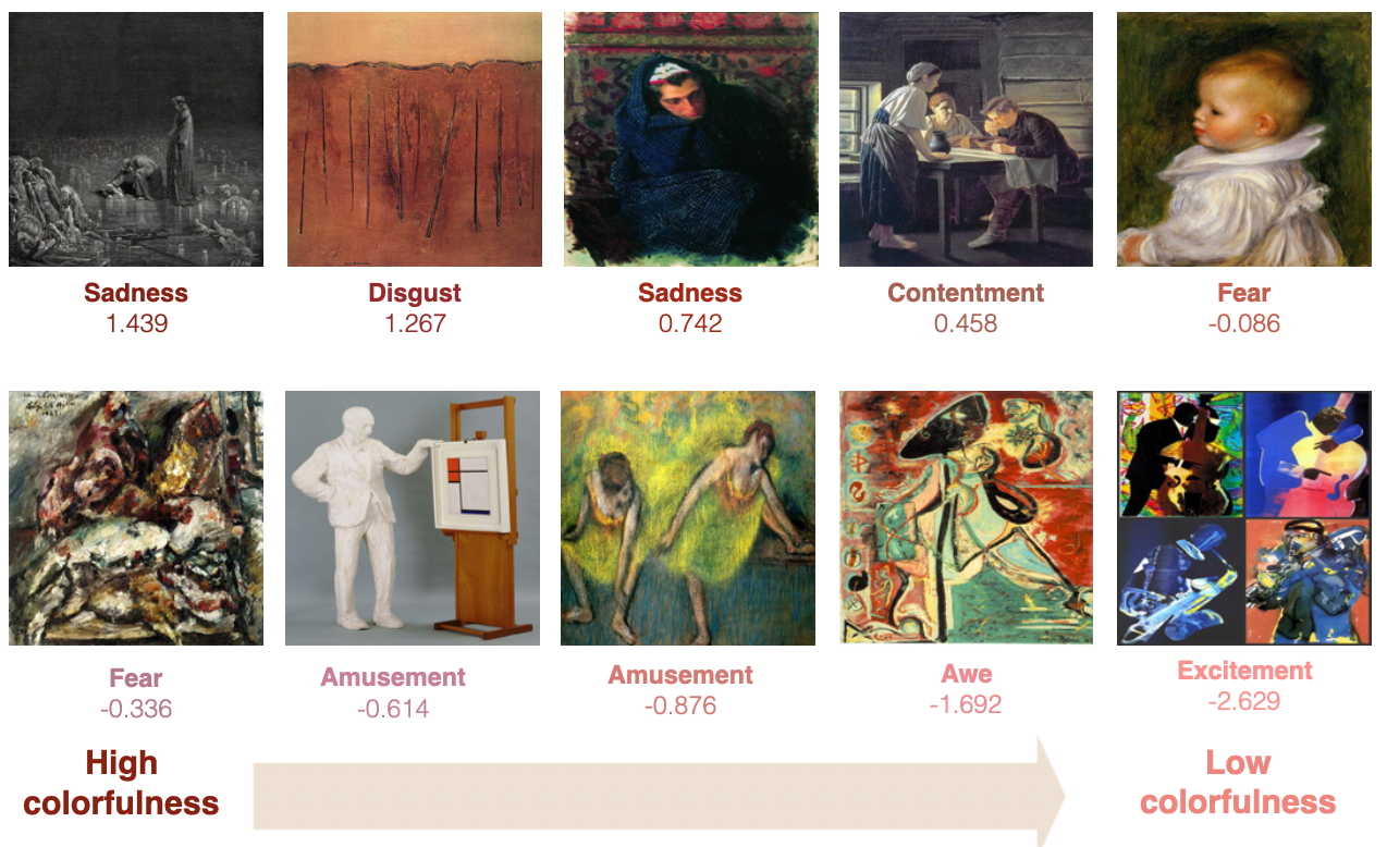
Colorfulness measures the Earth Mover’s Distance between the histogram of the painting and the histogram having a uniform color distribution. Images are converted into the CIE-Lab color space and 3D pixel representation are clustered into bins in the histogram [17]. Paintings with high colorfulness values tend to be dominanted by a single color, and paintings with low colorfulness values tend use all colors uniformly. Figure 5 shows some paintings with their normalized colorfulness value. As can be seen in Figure 6, colorfulness is positively correlated with negative emotion.


Figure 5. Paintings from the ArtEmis dataset with their corresponding ground truth majority emotion, and their normalized colorfulness value.

Figure 6. Ground truth emotion label and normalized colorfulness value for 4000 points randomly sampled from the balanced binary Artemis dataset. We observe a negative correlation between colorfulness and positive emotion.


Correlation between handcrafted features and learned features

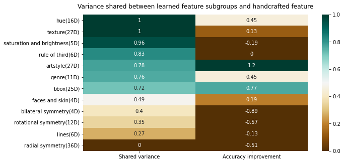
Figure 10 summarizes the correlation between handcrafted features and deep-learning based features. The first column in Figure 10 shows the proportion of variance shared between all canonical variates with significant correlation, which approximately informs us to what extent, the feature set with larger variance explains the feature set with smaller variance. As can be seen, some low-level features are almost completely explained by learned features, suggesting learned features almost completely encode these low-level information. On the other hand, there is less information overlap between learned features and handcrafted features on high-level variables such as artstyle, genre, and bboxes. Finally, some low-level features correlate weakly with learned features, possibly because the model did not pick up on these particular features during training.

The second column shows the improvement in a linear SVM classifier accuracy if we were to concatenate the handcrafted feature subgroup to the learned features, compared to only using learned features.

As shown in Figure 10, the strongly correlated handcrafted feature subgroups introduce no improvement to the SVM classifier, as expected. Moreover, the high-level feature subgroups, artstyle, genre and bounding boxes, are very helpful to the prediction task but the model did not fully learned them. Finally, low-level features subgroups rotational symmetry, lines, and radial symmetry, also introduce no improvement to the accuracy of the SVM classifier, suggesting that those features are not helpful to the task and are not learned by the deep model.

Figure 10. Column 1: Porportion of variance shared between canonical variates of learned features and handcrafted feature subgroups with significant correlation (>0.45). Column 2: Improvement in a linear SVM classifier accuracy if we were to concatenate the handcrafted feature subgroup to the learned features, compared to only using learned features.

Full list of handcrafted features

Scroll to see the full list of handcrafted features.

Category: 'saturation and brightness' (see [3])

  • 'mean saturation': mean saturation of the painting in HSY color space
  • 'mean brightness': mean brightness of the painting in HSY color space
  • 'pleasure': 0.69 Brightness +0.22 Saturation
  • 'arousal': −0.31 Brightness +0.60 Saturation
  • 'dominance': 0.76 Brightness +0.32 Saturation
  • Category: 'hue' (see [3])

  • 'saturation-weighted vector-based mean hue': Mean hue weighted by saturation
  • 'saturation-weighted angular dispersion': Angular dispersion weighted by saturation
  • 'vector-based mean hue': Mean hue.
  • 'angular dispersion': Mean angular dispersion of hue
  • 'colorfulness': Earth Mover’s Distance between the histogram of the painting and the histogram having a uniform color distribution,
  • 'black': Out of 11 basic colors, how many pixels are black
  • 'blue': Out of 11 basic colors, how many pixels are blue
  • 'brown':Out of 11 basic colors, how many pixels are brown
  • 'green':Out of 11 basic colors, how many pixels are green
  • 'gray':Out of 11 basic colors, how many pixels are gray
  • 'orange':Out of 11 basic colors, how many pixels are orange
  • 'pink':Out of 11 basic colors, how many pixels are pink
  • 'purple':Out of 11 basic colors, how many pixels are purple
  • 'red':Out of 11 basic colors, how many pixels are red
  • 'white':Out of 11 basic colors, how many pixels are white
  • 'yellow':Out of 11 basic colors, how many pixels are yellow
  • Category: 'texture' (see [3])

  • 'coarseness': coarseness from Tamura texture features
  • 'contrast': contrast from Tamura texture features
  • 'directionality': directionality from Tamura texture features
  • 'wavelet(level 1) hue': wavelet feature from level 1 of a three-level wavelet transform on the Hue channel.
  • 'wavelet(level 1) saturation': wavelet feature from level 1 of a three-level wavelet transform on the Saturation channel.
  • 'wavelet(level 1) brightness': wavelet feature from level 1 of a three-level wavelet transform on the Brightness channel.
  • 'wavelet(level 2) hue': wavelet feature from level 2 of a three-level wavelet transform on the Hue channel.
  • 'wavelet(level 2) saturation': wavelet feature from level 2 of a three-level wavelet transform on the Saturation channel.
  • 'wavelet(level 2) brightness': wavelet feature from level 2 of a three-level wavelet transform on the Brightness channel.
  • 'wavelet(level 3) hue': wavelet feature from level 3 of a three-level wavelet transform on the Hue channel.
  • 'wavelet(level 3) saturation': wavelet feature from level 3 of a three-level wavelet transform on the Saturation channel.
  • 'wavelet(level 3) brightness': wavelet feature from level 3 of a three-level wavelet transform on the Brightness channel.
  • 'wavelet(level 1)': The sum over level 1 Hue, Saturation and Brightness features
  • 'wavelet(level 2)': The sum over level 2 Hue, Saturation and Brightness features
  • 'wavelet(level 3)': The sum over level 3 Hue, Saturation and Brightness features
  • 'GLCM contrast (hue)': a measure of the hue contrast between a pixel and its neighbor over the whole image
  • 'GLCM contrast (saturation)': a measure of the saturation contrast between a pixel and its neighbor over the whole image
  • 'GLCM contrast (brightness)': a measure of the brightness contrast between a pixel and its neighbor over the whole image
  • 'GLCM correlation (hue)': statistical measure of how correlated a pixel's hue is to its neighbor's over the whole image. Range = [-1 1]. Correlation is 1 or -1 for a perfectly positively or negatively correlated image. Correlation is NaN for a constant image.
  • 'GLCM correlation (saturation)': statistical measure of how correlated a pixel's saturation is to its neighbor's over the whole image.
  • 'GLCM correlation (brightness)': statistical measure of how correlated a pixel's brightness is to its neighbor's over the whole image.
  • 'GLCM energy (hue)': summation of squared elements in the hue GLCM. Range = [0 1]. Energy is 1 for a constant image.
  • 'GLCM energy (saturation)': summation of squared elements in the saturation GLCM. Range = [0 1]. Energy is 1 for a constant image.
  • 'GLCM energy (brightness)': summation of squared elements in the brightness GLCM. Range = [0 1]. Energy is 1 for a constant image.
  • 'GLCM homogeneity (hue)': closeness of the distribution of elements in the hue GLCM to the hue GLCM diagonal.
  • 'GLCM homogeneity (saturation)': closeness of the distribution of elements in the saturation GLCM to the hue GLCM diagonal.
  • 'GLCM homogeneity (brightness)': closeness of the distribution of elements in the brightness GLCM to the hue GLCM diagonal.
  • Category: 'lines' (see [3])

  • 'static absolute line slopes': Average static line slope. Lines are extracted based on Hough Transform, static lines have slope less than 15 degrees.
  • 'static relative line slopes': Average static line slope relative to the closest axis.
  • 'length of static lines': Average length of static lines.
  • 'dynamic absolute line slopes': Average dynamic line slope, dynamic lines have slope larger than 15 degrees.
  • 'dynamic relative line slopes': Average dynamic line slope relative to the closest axis.
  • 'length of dynamic lines': Average length of dynamic lines.
  • Category: 'rule of third' (see [3])

  • 'mean hue of inner rectangle': mean hue of the inner rectangle, where painting is divided into 9 equal parts.
  • 'mean saturation of inner rectangle': mean saturation of the inner rectangle, where painting is divided into 9 equal parts.
  • 'mean brightness of inner rectangle':mean brightness of the inner rectangle, where painting is divided into 9 equal parts.
  • 'ratio of wavelet coef of inner rectgl vs. image. Hue': ratio of wavelet coefficients of inner rectangle vs. whole image, for the hue channel
  • 'ratio of wavelet coef of inner rectgl vs. image. Saturation': ratio of wavelet coefficients of inner rectangle vs. whole image, for the saturation channel
  • 'ratio of wavelet coef of inner rectgl vs. image. Brightness': ratio of wavelet coefficients of inner rectangle vs. whole image, for the brightness channel
  • Category: 'faces and skin' (see [3])

  • 'number of frontal faces': Number of faces detected in the image
  • 'relative size of the biggest face': size of the biggest face with respect to the image
  • 'number of skin pixels':the number of pixels in skin color
  • 'amount of skin wrt the size of faces': the proportion of the “skin area” to the size of the detected face
  • Category: 'bilateral symmetry' (see [9])

  • 'bilateral symmetry number': Number of symmetrical feature points involved in the maximum bilateral symmetry line,
  • 'bilateral symmetry radius': Radius of the maximum bilateral symmetry line (length of the norm in the Hough coordinate system),
  • 'bilateral symmetry angle': Angle of the maximum bilateral symmetry line in the Hough coordinate system,
  • 'bilateral symmetry strength': Normalized score of the maximum symmetry line in the maximum symmetry line voting procedure,
  • Category: 'rotational symmetry' (see [9])

  • 'rotational symmetry radius 1': Radius of the maximum rotational symmetry
  • rotational symmetry X coord 1': X coordinate of the maximum rotational symmetry
  • 'rotational symmetry Y coord 1': Y coordinate of the maximum rotational symmetry
  • 'rotational symmetry radius 2': Radius of the second maximum rotational symmetry
  • rotational symmetry X coord 2': X coordinate of the second maximum rotational symmetry
  • 'rotational symmetry Y coord 2': Y coordinate of the second maximum rotational symmetry
  • 'rotational symmetry radius 3': Radius of the third maximum rotational symmetry
  • rotational symmetry X coord 3': X coordinate of the third maximum rotational symmetry
  • 'rotational symmetry Y coord 3': Y coordinate of the third maximum rotational symmetry
  • Category: 'radial symmetry' (see [9])

  • 'radial symmetry map distribution 0' to 'radial symmetry map distribution 35': Each of the 36 features is one component in the distribution of symmetry map after radial symmetry transformation.
  • Category: 'genre'

  • 'genre_is_missing': Genre of the painting is missing
  • 'genre_is_portrait': Genre of the painting is portrait, according to WikiArt
  • 'genre_is_landscape': Genre of the painting is landscape, according to WikiArt
  • 'genre_is_still_life': Genre of the painting is still life, according to WikiArt
  • 'genre_is_religious_painting': Genre of the painting is religious painting, according to WikiArt
  • 'genre_is_sketch_and_study': Genre of the painting is sketch and study, according to WikiArt
  • 'genre_is_genre_painting': Genre of the painting is genre painting, according to WikiArt
  • 'genre_is_illustration': Genre of the painting is illustration, according to WikiArt
  • 'genre_is_cityscape': Genre of the painting is cityscape, according to WikiArt
  • 'genre_is_nude_painting': Genre of the painting is nude painting, according to WikiArt
  • 'genre_is_abstract_painting': Genre of the painting is abstract painting, according to WikiArt
  • Category: 'artstyle'

  • 'artstyle_is_Post_Impressionism': Style of the painting is Post Impressionism, according to WikiArt
  • 'artstyle_is_Expressionism'
  • 'artstyle_is_Impressionism'
  • 'artstyle_is_Northern_Renaissance'
  • 'artstyle_is_Realism'
  • 'artstyle_is_Romanticism'
  • 'artstyle_is_Art_Nouveau_Modern'
  • 'artstyle_is_Symbolism'
  • 'artstyle_is_Baroque'
  • 'artstyle_is_Abstract_Expressionism'
  • 'artstyle_is_Naive_Art_Primitivism'
  • 'artstyle_is_Rococo'
  • 'artstyle_is_Cubism'
  • 'artstyle_is_Naive_Art_Primitivism'
  • 'artstyle_is_Pop_Art'
  • 'artstyle_is_Pointillism'
  • 'artstyle_is_Early_Renaissance'
  • 'artstyle_is_Ukiyo_e'
  • 'artstyle_is_Mannerism_Late_Renaissance'
  • 'artstyle_is_High_Renaissance'
  • 'artstyle_is_Minimalism'
  • 'artstyle_is_Fauvism'
  • 'artstyle_is_Action_painting'
  • 'artstyle_is_Contemporary_Realism'
  • 'artstyle_is_Synthetic_Cubism'
  • 'artstyle_is_New_Realism'
  • 'artstyle_is_Analytical_Cubism'
  • Category: 'score and coordinates of bounding boxes of person'

  • 'bbox PCA 0' to 'bbox PCA 24':
  • The raw bbox feature contains bounding boxes of person. It's a 50D vector with the first 10D consisting the scores of the top 10 bounding boxes, and the 40D consists of the corresponding coordinates. We finutuned Faster R-CNN on the PeopleArt dataset to extract the bounding boxes. The finetuned model can be downloaded from here We use PCA to reduce the 50D vector to 25D, while perserving 99% variance.

    References

    [1] Sartori, A., Yanulevskaya, V., Salah, A. A., Uijlings, J., Bruni, E., & Sebe, N. (2015). Affective analysis of professional and amateur abstract paintings using statistical analysis and art theory. ACM Transactions on Interactive Intelligent Systems (TiiS), 5(2), 1-27.

    [2] Lu, X., Suryanarayan, P., Adams Jr, R. B., Li, J., Newman, M. G., & Wang, J. Z. (2012, October). On shape and the computability of emotions. In Proceedings of the 20th ACM international conference on Multimedia (pp. 229-238).

    [3]Machajdik, J., & Hanbury, A. (2010, October). Affective image classification using features inspired by psychology and Art Theory. In Proceedings of the 18th ACM international conference on Multimedia (pp. 83-92).

    [4] Yanulevskaya, V., van Gemert, J. C., Roth, K., Herbold, A. K., Sebe, N., & Geusebroek, J. M. (2008, October). Emotional valence categorization using holistic image features. In 2008 15th IEEE international conference on Image Processing (pp. 101-104). IEEE.

    [5] Lee, J., Choi, J., & Seo, S. (2020). Emotion-inspired painterly rendering. IEEE Access, 8, 104565-104578.

    [6] Rao, T., Li, X., & Xu, M. (2020). Learning multi-level deep representations for image emotion classification. Neural Processing Letters, 51(3), 2043-2061.

    [7] Lu, X., Lin, Z., Jin, H., Yang, J., & Wang, J. Z. (2014, November). Rapid: Rating pictorial aesthetics using deep learning. In Proceedings of the 22nd ACM international conference on Multimedia (pp. 457-466).

    [8] You, Q., Luo, J., Jin, H., & Yang, J. (2016, February). Building a large scale dataset for image emotion recognition: The fine print and the benchmark. In Proceedings of the AAAI conference on artificial intelligence (Vol. 30, No. 1).

    [9] Zhao, S., Gao, Y., Jiang, X., Yao, H., Chua, T. S., & Sun, X. (2014, November). Exploring principles-of-art features for image emotion recognition. In Proceedings of the 22nd ACM international conference on Multimedia (pp. 47-56).

    [10] Kim, H. R., Kim, Y. S., Kim, S. J., & Lee, I. K. (2018). Building emotional machines: Recognizing image emotions through deep neural networks. IEEE Transactions on Multimedia, 20(11), 2980-2992.

    [11] Elgammal, A., Liu, B., Kim, D., Elhoseiny, M., & Mazzone, M. (2018, April). The shape of art history in the eyes of the machine. In Proceedings of the AAAI Conference on Artificial Intelligence (Vol. 32, No. 1).

    [12] Côté-Allard, U., Campbell, E., Phinyomark, A., Laviolette, F., Gosselin, B., & Scheme, E. (2020). Interpreting deep learning features for myoelectric control: A comparison with handcrafted features. Frontiers in bioengineering and biotechnology, 8, 158.

    [13] Achlioptas, P., Ovsjanikov, M., Haydarov, K., Elhoseiny, M., & Guibas, L. J. (2021). ArtEmis: Affective language for visual art. In Proceedings of the IEEE/CVF Conference on Computer Vision and Pattern Recognition (pp. 11569-11579).

    [14] Lundberg, S. M., & Lee, S. I. (2017, December). A unified approach to interpreting model predictions. In Proceedings of the 31st international conference on neural information processing systems (pp. 4768-4777).

    [15] Westlake, N., Cai, H., & Hall, P. (2016). Detecting People in Artwork with CNNs. In European Conference on Computer Vision (pp. 825–841).

    [16] Lu, X., Lin, Z., Jin, H., Yang, J., & Wang, J. Z. (2014, November). Rapid: Rating pictorial aesthetics using deep learning. In Proceedings of the 22nd ACM international conference on Multimedia (pp. 457-466).

    [17] Rubner, Y., Tomasi, C., & Guibas, L. J. (2000). The earth mover's distance as a metric for image retrieval. International journal of computer vision, 40(2), 99-121.